plotbridge: A template-based bridge between Python and your plot engine
With a plotbridge template, you can use your favorite plotting program for visualizing the results of your Python data analysis or simulation code. The purpose is to keep the Python side free of most formatting details, while allowing arbitrarily complex templates (and optional preprocessing steps) that can produce publication quality plots in an automated and repeatable way.
Plotbridge relies heavily on Jinja2 and, of course, the plot engines that the templates target.
Note
If you’re familiar with PHP, think of the template as the HTML + PHP markup, but with HTML replaced by your plot engine syntax (e.g., gnuplot) and PHP replaced by Jinja2.
Getting started
Without further ado, we give some basic examples below. See the Examples page for more.
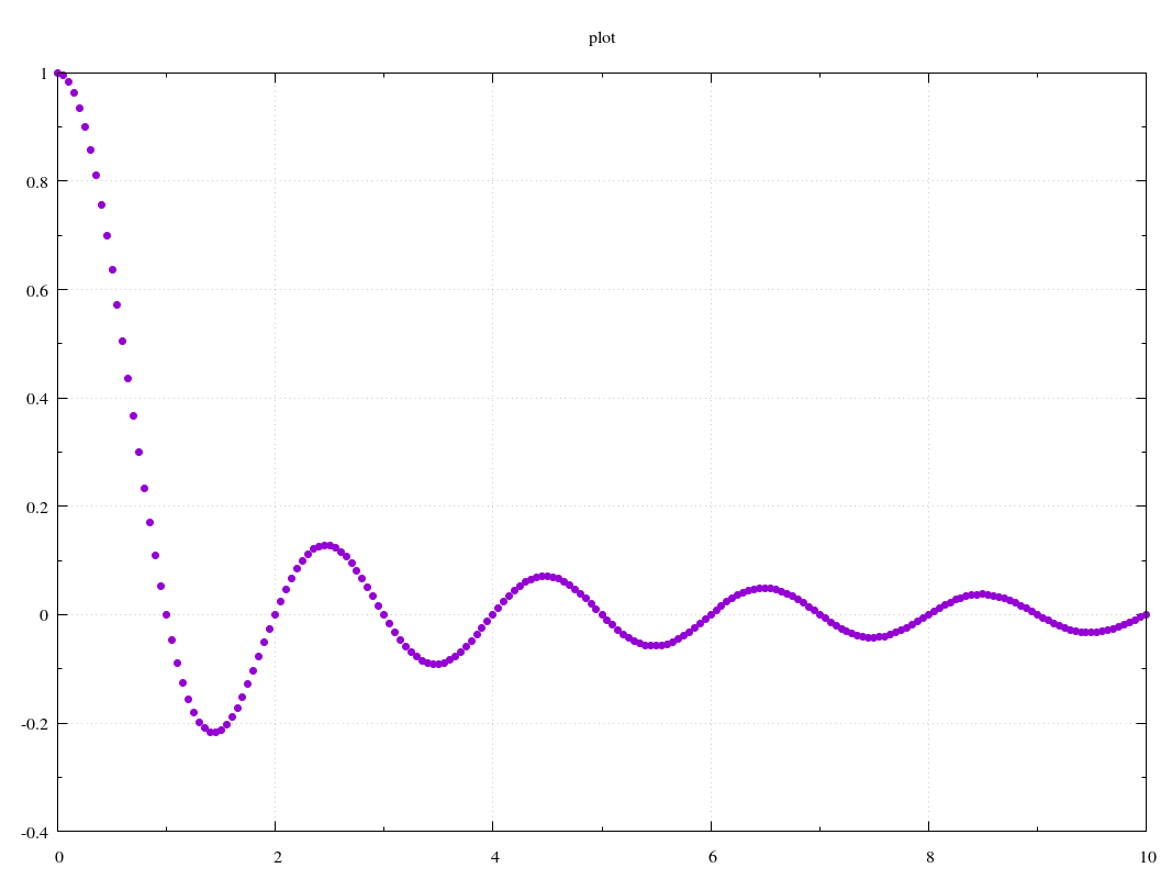
Hello, world!
A (near) minimal example from examples/gnuplot_minimal/minimal.py:
#!/usr/bin/python

from plotbridge.plot import Plot
import numpy as np

p = Plot() # by default, Plot uses
           #   template='gnuplot_2d', (plot) name="plot",
           #   output_dir='.', and overwrite=False

x = np.linspace(0,10,201)
p.add_trace(x, np.sinc(x))

# Generate the output (i.e., the .gnuplot script
# stored in <output_dir>/<plot_name>).
p.update()

# Run the plot engine (gnuplot), i.e., execute the
# plot script generated in the subdir "plot".
# Since the template was 'gnuplot_2d', this will only
# work if you have gnuplot installed!
p.run()
2D sweep
A typical (noisy) measurement as a function of two sweep parameters from examples/gnuplot_heatmap/heatmap.py:
#!/usr/bin/python

from plotbridge.plot import Plot
import numpy as np
np.random.seed(123) # makes automated testing easier

p = Plot('Transmission vs f and B',
         template='gnuplot_2d_stacked_image',
         overwrite=True)

p.set_width(400)
p.set_height(300)
p.set_xlabel('frequency (GHz)'); p.set_xunits(1e9)
p.set_ylabel('B field (mT)'); p.set_yunits(1e-3)
p.set_zlabel('S_{21}')
p.set_zlog(True)
p.set_grid(False)

for bfield in np.linspace(-.9e-3, .9e-3, 51):
  f0 = 1.3e9 - 1e9*np.abs(bfield/1e-3)**2
  w = 30e6
  freq = np.linspace(f0 - 400e6, f0 + 400e6, 101) # Hz
  transmission = 1 / ( 1 + (2*(freq-f0)/w)**2 ) # fake data
  transmission += np.abs( 0.02 * np.random.randn(len(transmission)) ) # fake noise
  p.add_trace(freq, transmission,
              slowcoordinate=bfield)

p.set_xrange(0.4, 1.6) # None, None --> autorange
p.set_yrange(-.8, .8)
p.set_zrange(1e-3, 1.05)

p.update()
p.run()

Templates
The inputs to plotbridge are (a) the data points and basic plot options from Python and (b) a template from a text file. Optionally, you can include a preprocess script (e.g. in Python) that massages the data before passing it to your plotting program.
For example, the gnuplot_2d template is defined by the files
in the directory default_templates/gnuplot_2d (and the
common_helper_scripts directory):
gnuplot_2d.template– the main template as gnuplot + jinja2 markupgnuplot_2d.cfg– a config file for miscellaneous settingsgnuplot.interactive.py– an optional script that runs the plot interactively (if different from running the plot script directly).
Note
Common scripts shared by many templates (such as
gnuplot.interactive.py) reside in the
common_helper_scripts directory, instead of the template
directory.
Some templates are provided in the default_templates directory.
They are great for your initial quick-and-dirty plots.
However, you’ll want a custom template for the vast majority of
published plots. The easiest way to do this is to copy one of the
directories from the default_templates directory to your
working directory, rename it, change the template=... argument
to plot.Plot.__init__() to the same name, and start hacking.
Note
The names of the .template and the .cfg,
files must match the name of the template directory. The names of
the (optional) .preprocess and .interactive.py files
are specified in the .cfg file.
Note
In addition to the standard files, you can have arbitrary
files in the template. They will all be copied to the plot directory
upon calling plot.Plot.__init__().
What templates look like
Here are some example statements you might find a typical (gnuplot)
.template file:
{% if global_opts.ylabel %}
set ylabel "{{ global_opts.ylabel }}" offset -1,0
{% endif %}
...

{% if global_opts.xlog %}
set logscale x
{% endif %}
...

{% if not global_opts.xrange|allnone %}
set xrange [{{ global_opts.xrange[0]|ifnone('') }}:{{ global_opts.xrange[1]|ifnone('') }}]
{% endif %}
...

plot \
{% for trace in traces %}
 ...
 linetype {{ trace.linetype|ifnone(1) }} \
 ...
{% endfor %}
If you wanted to, say, move the y-axis label a tiny bit to the left
and up, you could change the offset -1,0 to offset
-1.5,1. That’s the power of custom templates: you can control the
finest formatting details while keeping the Python interface simple.
If you wanted to create a template for your favorite plot engine, you
would simply replace the gnuplot commands by the appropriate commands
(e.g., for Matlab, set(ax,'XScale','log'); instead of
set logscale x).
The variables available in the templates consist of (a) the plot-level
global_opts specified with the set_* methods of the
plot.Plot class and (b) the per-trace trace.* options
passed to plot.Plot.add_trace().
Note
The include Jinja2 statement is handy for
reusing template fragments in multiple templates. You can include
any file in your template directory or in the default
template_fragments directory.
Note
You can also use Jinja2’s built-in template inheritance, which allows for more sophisticated nesting of templates. However, in that case you would specify the references in the “opposite direction,” i.e., one base template would define the overall structure with placeholder blocks that different child templates would fill in differently.
Template configuration file (.cfg)
The .cfg file specifies miscellaneous template options:
- extension – Extension of the main plot file (e.g.
.gnuplot). - executable – Mark the generated plot script as directly executable (N/A to Windows)?
- interactive-script – (Optional) name of a script that creates an
interactive version of the plot
(e.g.
gnuplot.interactive.py). Just the extension is enough if the file is in the template directory. If no match is found in the template directory, thecommon_helper_scriptsdirectory is also searched. - preprocess-script – Same as interactive-script, but for the (optional) preprocess script.
- preprocess-timeout – Max. number of seconds given to preprocess script to finish (specify as an integer).
- interpreter – If not empty, pass the output plot script
(e.g.
myplot.gnuplot) as an argument to the interpreter (e.g.gnuplot). - interactive-interpreter – If not empty, pass the interactive script
(e.g.
gnuplot.interactive.py) as an argument to the interpreter (e.g.python). - preprocess-interpreter – If not empty, pass the preprocess script
(e.g.
gnuplot_2d_stacked_image.preprocess) as an argument to the interpreter (e.g.python). - export-formats – A space separated list of available export
formats (e.g.
png pdf).
Plots
Once a plot is generated from the template, the output directory is
fully independent of the template and the code that generated it. For
example, the plot subdirectory generated by minimal.py
above contains:
plot.gnuplot– The main plot script produced fromgnuplot_2d.template.trace_UUID1.bytes– Binary data for trace 1 (referenced inplot.gnuplot).gnuplot_2d.interactive.py– A copy from the template directory. Callingplot.Plot.run()executes this.gnuplot_2d.interactive.py.out– Textual output from the script above. Check this if the plot does not pop up after callingplot.Plot.run().output.png– Generated after callingplot.Plot.run().
You can modify plot.gnuplot, move the directory elsewhere, or
re-execute gnuplot_2d.interactive.py to your heart’s
content. However, it’s usually smarter to create a custom template and
modify that instead, unless you’re absolutely sure you won’t need to
update the data points later.
Warning
If you do modify the output directory, watch out for your
original Python process (if it’s still running) calling
plot.Plot.update(). That overwrites plot.gnuplot!
Similarly, calling plot.Plot.__init__() with
overwrite=True and the same name and
output_dir will erase all contents of the plot directory!
In the wild
Plotbridge is used (at least) in:
- qtlab – a Python framework for running computer-controlled experiments.
- J. Govenius et al., “Parity measurement of remote qubits using dispersive coupling and photodetection,” Phys. Rev. A 92, 042305 (2015) (open access).
- J. Govenius et al., “Detection of zeptojoule microwave pulses using electrothermal feedback in proximity-induced Josephson junctions,” Phys. Rev. Lett. 117, 030802, (2016) (open access).